
- SPEECH
Determinants of the real interest rate
Remarks by Philip R. Lane, Member of the Executive Board of the ECB, at the National Treasury Management Agency
Dublin, 28 November 2019
Introduction
It is a pleasure to address the Annual Investee and Business Leaders’ Dinner organised by the National Treasury Management Agency (NTMA).[1] I plan today to explore some of the factors determining the evolution of the real (that is, inflation-adjusted) interest rate over time.
This is obviously relevant to the NTMA in its role as manager of Ireland’s national debt and also to its other business areas (Ireland Strategic Investment Fund; State Claims Agency; NewEra; National Development Finance Agency) and related entities (National Asset Management Agency; Strategic Banking Corporation of Ireland; Home Building Finance Ireland). More generally, the real interest rate is at the core of many financial valuation models, while simultaneously acting as a fundamental macroeconomic adjustment mechanism by reconciling desired savings and desired investment patterns.
My primary focus today is on the real interest rate on sovereign bonds, which in turn is the baseline for pricing riskier bonds and equities through the addition of various risk premia. The real return on government bonds in advanced economies has undergone pronounced shifts over time. Chart 1 shows that, since the 1980s, the real return on sovereign debt has registered a steady decline towards levels that are low from a historical perspective. Looking at the 1970s, ex-post calculations of the real interest rate were also low during this period, since inflation turned out to be unexpectedly high. In contrast, the current low levels of the real interest rate take the form of low nominal yields, since inflation is itself low and stable.[2] Understanding the root causes of the low level of real interest rates is a high priority for monetary and fiscal policymakers, financial-sector participants and the wider populations of savers and investors.
Chart 1
Real ten-year sovereign bond yields
(percentages per annum)
Sources: IMF, FRED, Thomson Reuters, ECB staff calculations and Jordà, Ò., Knoll, K., Kuvshinov, D., Schularick, M. and Taylor, A. M. (2019), “The Rate of Return on Everything, 1870-2015”, The Quarterly Journal of Economics, Vol. 134, No 3, pp. 1225-1298.
Notes: Real sovereign bond yields are calculated as the difference between the nominal yield in year t and realised inflation in year t. The euro area series is based on GDP-weighted data for Germany, France, Italy and Spain. Data for Italy before 1991, for Spain before 1980 and for Germany, France and the United States before 1973 are based on Jordà et al. (2019), op. cit.
Latest observation: 2019.
The natural rate of interest
The falling trend in yields can be interpreted as a decline in the so-called natural or neutral rate of interest (labelled as r* in academic research and policy discussions). The natural rate of interest corresponds to the level of the real short-term interest rate that defines a neutral policy stance: this corresponds to a situation in which the economy is operating at potential and inflation is at its target value, such that there is no reason for the central bank to either inject or withdraw stimulus.
In what follows I will explore the causes of this trend decline in r*.
Causes of the persistent low real yield environment
I will structure my discussion of the drivers of r* around three broad driving forces: first, the determinants of potential growth rates; second, demographics; and third, diverging developments in the returns on risky and safe financial assets.[3] These three factors are embedded in the textbook economic growth model, which relates the equilibrium rate of interest to economic growth, population growth and the discount rate. I will primarily focus on common international trends, even if cross-country differences in these driving forces have important implications for return differentials and international capital flows.[4],[5]
The potential growth rate
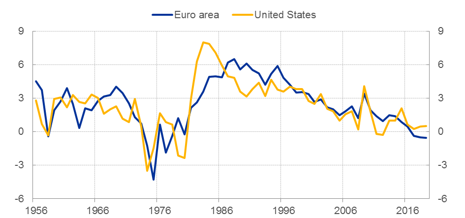
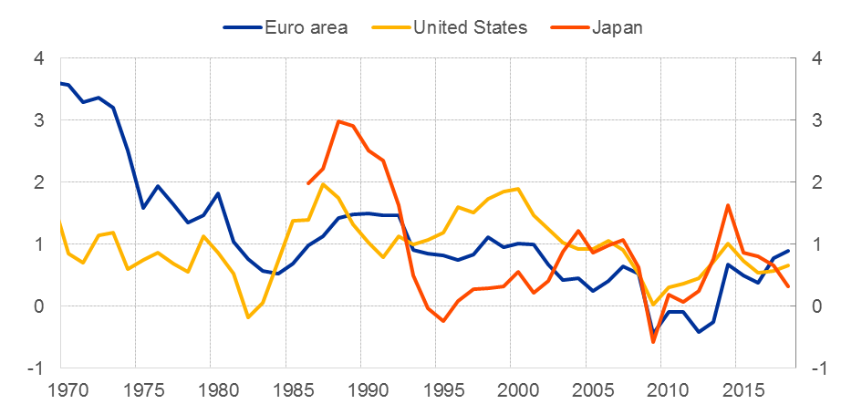
One fundamental driver of r* is the potential growth rate of the economy: in a high-growth economy, it takes a higher real interest rate to encourage the volume of saving required for the high investment levels needed to sustain a fast-growing economy. Although easier to see with the benefit of hindsight, there has been a sustained decline in the potential growth rate of advanced economies in recent decades: it is estimated to be less than half of what it was 50 years ago (Chart 2).[6] This pattern also carries over to expectations about future growth performance. The decline in potential output growth in turn can be attributed to a decline in total factor productivity growth (Chart 3) and a corresponding decline in labour productivity growth (Chart 4).[7]
Chart 2
Potential output growth and long-term growth expectations
(percentages per annum)

Sources: Bureau of Economic Analysis, European Commission and Consensus Economics.
Notes: The euro area data reflect the changing composition of Member States. The Consensus long-term growth estimates are for years t+6 to t+10. The first observation for Consensus long-term growth expectations is 1999 for the euro area and 1990 for the United States.
Latest observation: 2021 for euro area potential output growth estimates, 2019 for all other series.
Chart 3
Total factor productivity growth
(yearly growth rates, percentages, five-year moving averages, constant prices)
Sources: European Commission AMECO database and ECB staff calculations.
Notes: The euro area reflects data for the original 12 member states.
Latest observation: 2018.
Chart 4
Labour productivity: real gross value added per person employed
(yearly growth rates, percentages, five-year moving averages, constant prices)
Sources: European Commission AMECO database and ECB staff calculations.
Notes: The euro area reflects data for the original twelve Member States.
Latest observation: 2018.
A range of inter-related structural and technological factors have been advanced to explain the decline in the potential output growth rate. Assessing the determinants of the rate of technological innovation is beyond the scope of this speech.[8] In addition to the pace of frontier innovation, aggregate productivity growth also depends on the rate of technology diffusion. There are signs that the diffusion rate has slowed: for instance, the gap between the labour productivity growth of firms operating at the technology frontier in a given sector and that of firms that are lagging behind the technology frontier in that sector (non-frontier firms) has increased over time (Chart 5).[9] This pattern is even more pronounced in the services sector than in manufacturing.
Chart 5
Technology diffusion in manufacturing and services in the OECD and selected euro area countries
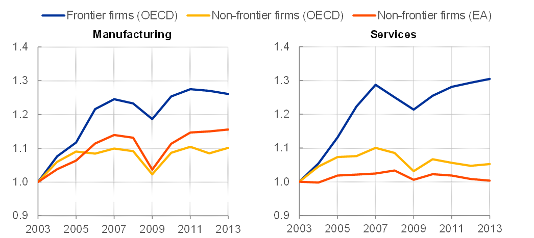
Sources: ECB staff calculations based on OECD data and the fifth vintage of CompNet data.
Notes: The OECD frontier and non-frontier productivity developments are taken from OECD (2015), The future of productivity. The productivity growth of the euro area is proxied as the unweighted average across Belgium, Spain, France, Italy and Finland of the median firm in each 1-digit sector (using the NACE Rev. 2 classification). NACE Rev.2 1-digit services sectors are then aggregated with value-added shares.
Latest observation: 2013.
This, of course, raises the question of why technological diffusion has slowed down. One candidate is the fall in business dynamism as measured by business churn: the rate at which firms exiting the market are replaced by new ones has declined measurably over the last decade (Chart 6).
Chart 6
Business churn in the euro area and United States
(sum of the birth and death rates of firms)

Sources: Eurostat and United States Business Dynamics Statistics.
Note: The euro area is represented by Belgium, Germany, Spain, France, Italy, Luxembourg, the Netherlands, Austria, Portugal, Slovenia and Finland.
Latest observation: 2016.
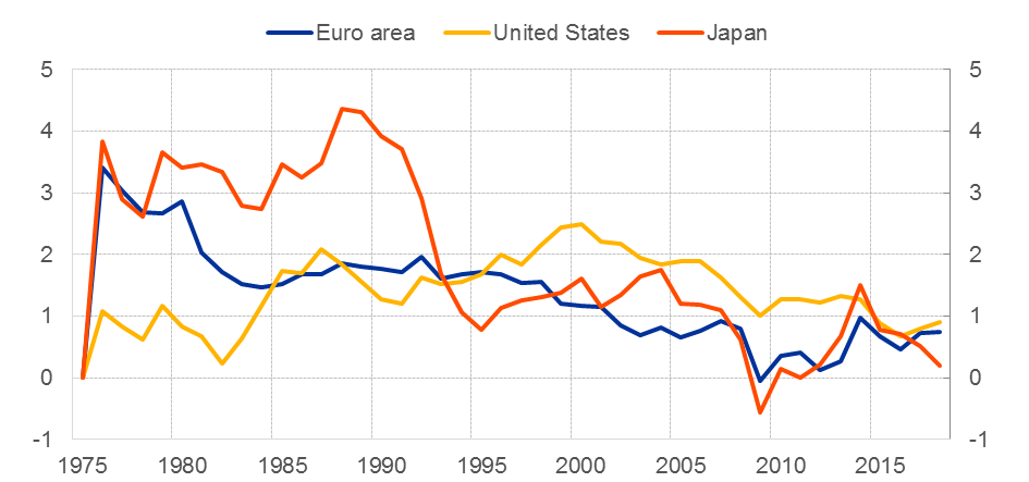
Finally, shifts in the sectoral distribution of economic activity also play a role. Employment growth has been concentrated in the services sector in recent years, and productivity growth in services has been weaker than in other sectors, such as manufacturing and information technology. As a result, the growing share of services in total employment mechanically implies a drag on productivity growth in the economy as a whole (Chart 7).
Assuming that the structural shifts I have just described account for a loss in potential output growth of around 1 percent, a back of the envelope calculation suggests that these account for a decline in real equilibrium yields of a similar magnitude.
Looking ahead, it is difficult to predict whether these structural trends will be reversed. In particular, there is a wide range of views about the potential economic impact of digitalisation, automation and artificial intelligence, which depends on the success rate in converting new technologies into economically-successful business applications. In turn, aggregate investment dynamics will be heavily influenced by this discovery process.
Another open question relates to climate change and the carbon transition. On the one side, future productivity growth may be further depressed as a consequence of climate change – either directly due to natural disasters or indirectly due to required climate change mitigation measures. On the other side, the carbon transition is also a spur for investment and opens up new opportunities for innovation and productivity growth.[10]
Chart 7
Euro area labour productivity by sector: real gross value added per person employed
(yearly growth rates, percentages, five-year moving averages, constant prices)

Sources: European Commission AMECO database and ECB staff calculations.
Notes: The euro area reflects data for the original 12 Member States.
Latest observation: 2018.
Demographics
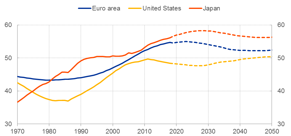
Let me now turn to a second driving force for the real interest rate: demography. Over the last 50 years, demographics in advanced economies have been characterised by low fertility rates and rising life expectancy (Chart 8). As a result, people now expect to enjoy many more years in retirement than they did in the 1970s, as Chart 9 shows for the euro area. Similarly, while in the 1970s and 1980s, the ratio of the elderly (aged 65 and over) to the working-age population (aged 15-64) was around 20 percent, the European Commission projects the old age dependency ratio will rise to over 50 percent by the middle of this century (Chart 10), while the ratio of older workers relative to younger workers has trended up significantly over the last decades (Chart 11). Over the same period, the annual growth rate of the working-age population has fallen from over 1 percent to zero and is projected to turn negative (Chart 12).
Chart 8
Life expectancy at birth: historical data and projections
(number of years)
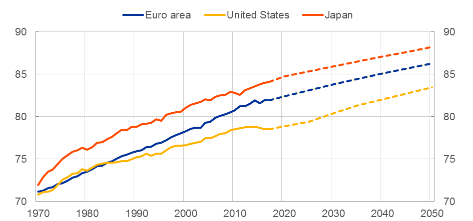
Source: World Bank.
Notes: Annual data. Dashed lines denote projected values. Projections begin in 2018.
Latest observation: 2017 for historical data and 2050 for projections.
Chart 9
Expected number of years spent in retirement for the largest euro area countries
(number of years)
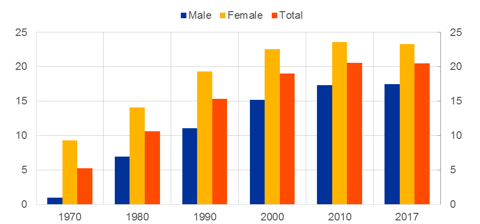
Sources: World Bank, United Nations, Eurostat, OECD and ECB staff calculations.
Notes: The chart reflects the difference between life expectancy at birth in year t and the effective retirement age in year t. The chart is a population-weighted average for Germany, France, Italy and Spain.
Latest observation: 2017.
Chart 10
Old-age dependency ratios: historical data and projections
(ratios)

Sources: World Bank, Eurostat, OECD and ECB staff calculations.
Notes: Dashed lines denote projected values. For the euro area, historical data are from the World Bank and projections are from Eurostat. All other historical data and projections are from the OECD.
Latest observation: 2018 for historical data and 2050 for projections.
Chart 11
Older worker ratio: ratio of 40-64 year olds over 15-64 year olds
(ratios)
Sources: World Bank, Eurostat, OECD and ECB staff calculations.
Notes: Dashed lines denote data points based on projected values. For the euro area, historical data are from the World Bank and projections are from Eurostat. All other historical data and projections are from the OECD.
Latest observation: 2018 for historical data and 2050 for projections.
Chart 12
Working-age population growth: historical data and projections
(year-on-year growth rates)

Sources: World Bank and ECB staff calculations.
Notes: Annual data. Dashed lines denote projected values. Projections begin in 2018.
Latest observation: 2017 for historical data and 2050 for projections.
But how do these demographic trends – which are without precedent – affect the equilibrium interest rate?
A number of mechanisms are at play. First, the ageing of the population can depress the demand for capital. This in turn is due to the fact that the ratio of installed capital relative to the size of the work force increases as the population ages. Second, ageing can lower productivity growth and thereby reduce investment opportunities. This materialises if the productivity of older age cohorts is lower than that of younger age cohorts. Third, in relation to savings rates, if rising life expectancy implies longer retirement periods then individuals and those responsible for publicly provided pensions face incentives to save more. Taken together, a lower level of desired investment and a higher level of desired saving imply a reduction in the natural rate of interest.
Some observers have conjectured that the negative impact of ageing on the equilibrium real rate will be reversed once the largest age cohorts retire and begin dissaving.[11] However, the increase in the capital-labour ratio associated with a sustained phase of higher saving and a contraction in the workforce will weigh on the level of real interest rates for a considerable time.[12]
In terms of magnitude, a wide range of estimates suggest that the downward impact on equilibrium real rates from slowing population growth and rising life expectancy over the period from 1980 to 2050 amounts to about 1 to 2 percentage points in both the United States and the euro area.[13]
While demographics constitute a powerful inter-generational influence on aggregate savings, the intra-generational distribution of income also matters. Chart 13 shows that the share of national income earned by households in the top 1 percent income bracket has increased considerably since the 1980s, both in the euro area and, even more strongly, in the United States. Assuming that the propensity to consume out of income is lower for rich households than for those with lower income and wealth, greater inequality may be associated with an increase in savings and further downward pressure on the real interest rate.[14]
Chart 13
Share of national income: top 1 percent
(percentages)

Source: World Inequality Database.
Notes: Pre-tax national income share held by a given percentile group. Pre-tax national income is the sum of all pre-tax personal income flows accruing to the owners of the production factors, labour and capital, before taking into account the operation of the tax/transfer system, but after taking into account the operation of pension system. The central difference between personal factor income and pre-tax income is the treatment of pensions, which are counted on a contribution basis by factor income and on a distribution basis by pre-tax income. The population is comprised of individuals over age 20. The base unit is the tax unit defined by national fiscal administrations to measure personal income taxes. The first observation is 1970 for Japan and the United States, and 1980 for the European Union.
Latest observation: 2017 for European Union, 2014 for United States and 2010 for Japan.
Diverging trends in the return on capital and on safe financial assets
A further complication relates to shifts in the relation between the return on so-called safe assets (such as highly-rated sovereign bonds) and wider measures of rates of return, including equity returns and returns on higher-risk debt instruments.[15] In related fashion, there has also been a shift in the relation between the returns on short-term instruments and those on longer-term instruments, with term premia that are much smaller now than in earlier periods (or even negative).[16]
On the one side, we have observed that corporate bond spreads have held up and estimates of the equity risk premium have increased, in both the United States and the euro area (Chart 14). On the other, the demand for short-term money-like instruments has surged, and the yield on those instruments has dropped to unprecedented negative values.
Chart 14
Corporate bond spreads and equity risk premium
(percentages)
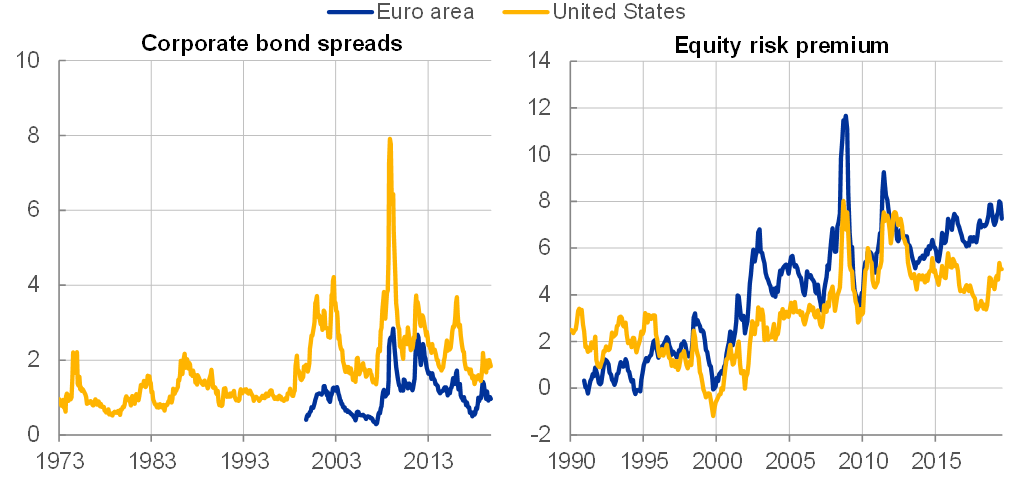
Sources: For corporate bond spreads – Merrill Lynch, ECB staff calculations and Gilchrist, S. and Zakrajšek, E. (2012), “Credit spreads and business cycle fluctuations”, American Economic Review, Vol. 102, No 4, pp. 1692-1720; for equity risk premium – Thomson Reuters, Consensus and ECB staff calculations.
Notes: Corporate bond spreads for the United States before 2010 are based on Gilchrist, S. and E. Zakrajšek (2012), ibid. Owing to historical data constraints, the equity risk premium is approximated by subtracting the real risk-free rate from the earnings yield.
Latest observation: October 2019.
A vibrant field of research seeks to reconcile the observed divergence in rates of return across asset categories with reference to shifts in mark-ups and risk premia.[17] This literature also highlights the increasing value attached to safe assets that offer protection against downside risks.[18]
The premium on safe assets is due to several inter-related factors, with the relative importance of individual factors shifting over time. First, ageing may play a role in moving portfolio preferences towards lower-risk assets, with older savers seeking safer income streams as retirement approaches. Second, at a global level, the accumulation of reserve-currency low-risk assets has been a central strategy for many emerging economies, in seeking to limit financial fragilities associated with a lack of foreign-currency liquidity.[19] However, this force has plausibly weakened in recent years, due to the strengthening of domestic-currency financial systems in many emerging markets and the adoption of more flexible exchange-rate regimes.
Third, the safety premium also reflects the lingering effects of the global financial crisis and the euro area sovereign debt crisis (Chart 15). By revealing the harsh costs of exposure to financial disasters, such crises tend to shift portfolio preferences in the direction of assets that preserve their value during bad times. In a similar vein, in recognition of the fact that the pre-crisis financial system was not sufficiently capitalised (compared with risk exposures) and not sufficiently liquid, regulatory reforms have also fuelled demand for safe assets, since banks have a reduced risk appetite and are also required to hold more liquid assets.[20]
Chart 15
Ten-year euro area sovereign bond yield to OIS spread
(basis points)
Source: Bloomberg and ECB staff calculations.
Note: Daily data.
Latest observation: 27 November 2019.
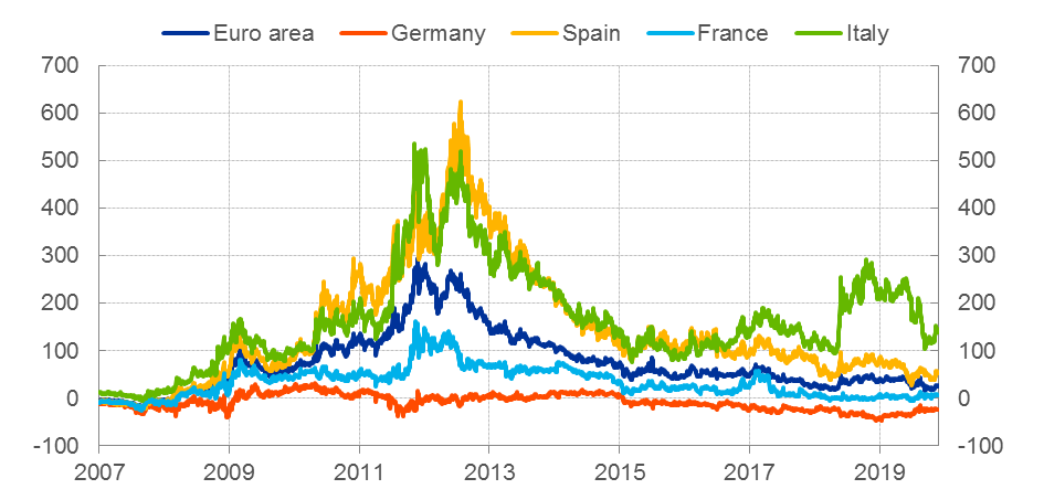
In terms of the supply of safe assets, the surge in public debt in the wake of the crisis and the operation of the doom loop between the risk profiles of banking systems and sovereigns has led to a relative contraction in the share of highly-rated sovereign bonds in the euro area. The share of government bonds in the euro area with AAA-rating from at least two rating agencies collapsed by two thirds and has become more concentrated (Chart 16). In the euro area the ratio of highly-rated short-term assets relative to GDP appears low in international comparison (Chart 17). More generally, safe asset scarcity tends to be most visible in yields on assets that provide the best hedge against liquidity, interest rate, or default risk (Chart 18).[21],[22]
Chart 16
Share of euro area sovereign bonds with AAA rating
(left-hand scale: percentages; right-hand scale: number of sovereign issuers)

Source: ECB.
Note: Ratings based on Moody’s, Fitch, Standard & Poor’s and DBRS.
Latest observation: 15 October 2019.
Chart 17
Share of short-term government debt with AAA rating relative to GDP
(percentages)
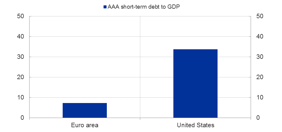
Source: ECB and US Treasury.
Notes: Ratings based on Moody’s, Fitch, Standard & Poor’s and DBRS. AAA-rating based on at least one of its ratings being AAA. Short-term debt refers to securities with a residual maturity of up to and including 2 years.
Latest observation: 15 October 2019 for government debt, end 2017 for GDP.
Chart 18
Two-year German government bond yield to OIS spread
(basis points)
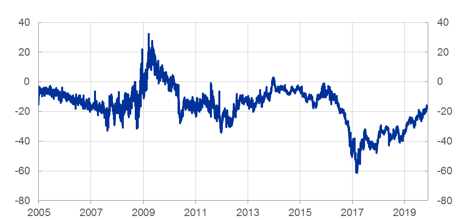
Sources: Thomson Reuters and ECB staff calculations.
Note: Daily data.
Latest observation: 27 November 2019.
Empirical Summary
The decline in potential growth rates, demographic trends and the portfolio shift towards safe assets combine to put downward pressure on the equilibrium real rate of interest. This rate is not directly observable: at any given point in time, temporary factors push the economy away from its underlying steady state so that the measured real interest rate also reflects these shocks (and the associated policy responses). However, analysis by the ESCB Working Group on Econometric Modelling indicates that, taking the impact of these driving factors into account, the equilibrium real interest rate in the euro area has been around zero or negative in recent years (Chart 19).[23] Similar estimates are reported in the growing literature on the global equilibrium real interest rate.[24] While Chart 19 shows that estimates of r* are inevitably not very precise, the general downward drift is quite clear.
Chart 19
Range of point estimates of the natural rate of interest in the euro area obtained from econometric models
(percentages)
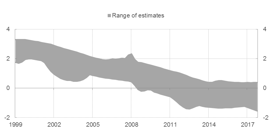
Notes: The grey-shaded area reports ranges of point estimates of r* for the euro area, as estimated in Brand, C. and Mazelis, F. (2019), “Taylor-rule consistent estimates of the natural rate of interest”, Working Paper Series, No 2257, ECB. Corresponding individual point estimates are reported in Brand, C. et al. (2019), op. cit.
Sources: Fiorentini, G., Galesi, A., Pérez-Quirós, G. and Sentana, E. (2018), “The Rise and Fall of the Natural Interest Rate,” Documentos de Trabajo, No 1822, Banco de Espanã; Hledik, T. and Vlcek, J. (2018), “Multi-country Model of the Euro Area,” Czech National Bank, forthcoming; Holston, K., Laubach, T. and Williams, J. C. (2017), “Measuring the natural rate of interest: International trends and determinants,” Journal of International Economics, Vol. 108, No S1, pp. 59-75; Jarocinski, M. (2017), “VAR-based estimation of the euro area natural rate of interest,” ECB Draft Paper.
Sample period: 1999 Q1 to 2017 Q4.
Policy Issues
What are the implications of low equilibrium real rates for policy?
Taking monetary policy first, it is important to recognise that the primary determinants of long-term equilibrium real rates are non-monetary in nature: potential growth rates; demographics; risk preferences in portfolios. Nonetheless, the implications of the level of real interest rates for the formulation of monetary policy are profound. In particular, monetary policy ultimately has to be calibrated vis-à-vis the underlying equilibrium rate of interest. If, for example, inflation stabilisation calls for monetary stimulus due to a negative demand shock, the central bank is required to engineer an easing of financial conditions relative to the steady state. If the prevailing inflation rate falls short of the inflation aim and the equilibrium real rate is low – or even negative – this may call for a substantially negative policy rate in order to stabilise medium-term inflation.
Furthermore, if the policy rate is already close to the effective lower bound, alternative methods of providing monetary stimulus may be required to substitute for deeper rate cuts. For example, a 1 percentage point decline in steady-state inflation translates into an equivalent loss of capacity to cut the policy rate in the event of an adverse shock: this is a large magnitude, given standard calculations of the monetary easing required during downturns in order to stabilise inflation over the medium term. Options to ease monetary policy when the conventional policy space is constrained include forward guidance about the future path of policy rates; asset purchase programmes; and targeted lending operations. Since the summer of 2014, the ECB has been active in employing all of these instruments and our assessment is that these unconventional policy measures have been highly effective in easing monetary and financial conditions.[25] At the same time, to avoid that the effective lower bound constrains monetary policy too frequently – and thus to reduce the need for unconventional policy tools – it is essential that inflation is centred at its target over the medium term, so that the limitations imposed by a low equilibrium real rate are not further compounded by an inflation trend that is also too low.
In relation to other policy dimensions, a low equilibrium real rate reflects – as I discussed earlier – low expected potential growth rates. It follows that growth-enhancing structural policies and growth-optimising public investment rates would translate into an upward shift in the equilibrium real rate. In addition, population ageing poses many policy challenges, and the policy choices that are made will have significant implications for trend savings and investment rates. In addition, in the event of negative shocks, the speed of convergence back to steady state can be accelerated if macroeconomic stabilisation is supported by counter-cyclical fiscal policies (where feasible) in addition to the stabilisation policies of central banks.
In addressing the safe-asset premium, policies that reduce negative tail risk are essential. Much has been done in the aftermath of the crisis to mitigate tail risks, especially in relation to the financial system: bank capitalisation levels have been increased, reinforced by an additional layer of loss-absorbing debt instruments; supervisory oversight has been enhanced, including through the creation of the Single Supervisory Mechanism; macroprudential policy frameworks have been initiated; macro-financial imbalances are more contained; and the European Stability Mechanism is a source of stability in the sovereign debt market. Still, it is also clear that the current system for bearing risk remains far from optimal, with the completion of banking union and the deepening of capital markets union offering much potential for risk sharing. In turn, a greater degree of risk sharing reduces the need for individual entities to self-insure through the accumulation of safe assets.
On the supply side, the sustained through-the-cycle maintenance of fiscal discipline (in combination with an active role for counter-cyclical fiscal stabilisation policies, which can help maintain the equilibrium real rate at a higher level) will over time lead to an improvement in the risk assessments of the national sovereign debt of euro area countries.[26] In addition, the supply of safe assets could be boosted at the euro area level through a range of innovations, even if some of these proposals require a significant deepening of fiscal union at the area-wide level.[27]
- I am grateful for the contribution by Claus Brand and Danielle Kedan to this speech.
- For a discussion of the evolution of nominal interest rates, see Lane, P. R. (2019), “The yield curve and monetary policy”, speech at the Centre for Finance and the Department of Economics at University College London, 25 November, London.
- A related, though not identical, approach has also been repeatedly suggested by James Bullard. See, for example, Bullard, J. (2019), “The Monetary Policy Implications of a Low R-Star: An Update”, presentation at the Joint DNB/ECB Workshop on the Natural Rate of Interest, 16 May, Amsterdam.
- See Lane, P. R. and Milesi-Ferretti, G. M. (2001), “Long-term capital movements”, NBER Working Paper Series, No 8366; and Higgins, M. (1998), “Demography, National Savings, and International Capital Flows”, International Economic Review, Vol. 39, No 2, pp. 343-369.
- See Kiley, M. T. (2019), “The Global Equilibrium Real Interest Rate: Concepts, Estimates, and Challenges”, forthcoming in the Annual Review of Financial Economics; Borio, C., Disyatat, P., Juselius, M. and Rungcharoenkitkul, P. (2017), “Why so low for so long? A long-term view of real interest rates”, BIS Working Paper, No 685, Bank for International Settlements; and Clarida, R. H. (2018), “The global factor in neutral policy rates: Some implications for exchange rates, monetary policy, and policy coordination”, BIS Working Paper, No 732, Bank for International Settlements.
- See Andersson, M., Szörfi, B., Tóth, M. and Zorell, N. (2018), “Potential output in the post-crisis period”, Economic Bulletin, Issue 7, ECB, pp. 49-70.
- See the European Investment Bank’s Investment Report 2019/2020 “Accelerating Europe’s transformation” released on 26 November 2019 for a discussion of the investment dynamics and financing in the European Union.
- Prominent contributions include: Gordon, R. J. (2017), The Rise and Fall of American Growth: The U.S. Standard of Living since the Civil War, Princeton University Press; Gordon, R. J. (2015), “Secular Stagnation: A Supply-Side View”, American Economic Review, Vol. 105, No 5, pp. 54-59; Summers, L. H. (2016), “The Age of Secular Stagnation: What It Is and What to do About It”, Foreign Affairs, Vol. 95, No 2; Summers, L. and Rachel, L. (2019) “On falling neutral real rates, fiscal policy, and the risk of secular stagnation”, Brookings Papers on Economic Activity, Spring 2019; Brynjolfsson, E. and McAfee, A. (2014), The Second Machine Age: Work, Progress, and Prosperity in a Time of Brilliant Technologies, WW Norton; Philippon, T. (2019), “The Great Reversal”, Harvard University Press; Bloom, N., Jones, C. I., Van Reenan, J. and Webb, M. (2019), “Are Ideas Getting Harder to Find?,” American Economic Review, forthcoming.
- See European Central Bank (2017), “The slowdown in euro area productivity in a global context”, Economic Bulletin, Issue 3, pp. 47-67.
- See Rudebusch, G. D. (2019), “Climate Change and the Federal Reserve”, FRBSF Economic Letter, 2019-09, Federal Reserve Bank of San Francisco; Batten, S., Sowerbutts, R. and Tanaka, M. (2016), “Let’s talk about the weather: the impact of climate change on central banks”, Staff Working Paper, No 603, Bank of England; and Acemoglu, D., Aghion, P., Barrage, L. and Hémous, D. (2019); “Climate Change, Directed Innovation, and Energy Transition: The Long-run Consequences of the Shale Gas Revolution”, Harvard University, mimeo.
- See Goodhart, C. and Pradhan, M. (2017), “Demographics will reverse three multi-decade global trends”, BIS Working Paper, No 656, Bank for International Settlements.
- See Lisack, N., Sajedi, R. and Thwaites, G. (2017), “Demographic trends and the real interest rate”, Staff Working Paper, No 701, Bank of England.
- See Bielecki, M., Brzoza-Brzezina, M. and Kolasa, M. (2018), “Demographics, monetary policy and the zero lower bound”, National Bank of Poland Working Paper, No 284; Papetti, A. (2019), “Demographics and the natural real interest rate: historical and projected paths for the euro area”, Working Paper Series, No 2258, ECB; Carvalho, C., Ferrero, A. and Nechio, F. (2016), “Demographics and real interest rates: Inspecting the mechanism”, European Economic Review, Vol. 88, pp. 208-226; Gagnon, E., Johannsen, B. K. and Lopez-Salido, D. (2016), “Understanding the New Normal: The Role of Demographics”, Finance and Economic Discussion Series, No 2016-080, Federal Reserve Board; Rachel, L. and Smith, T. D. (2015), “Secular drivers of the global real interest rate”, Staff Working Paper, No 571, Bank of England; Rachel, L. and Summers, L. H. (2019), “On Secular Stagnation in the Industrialized World”, NBER Working Paper Series, No 26198; and Jones, C. (2018), “Aging, Secular Stagnation and the Business Cycle”, IMF Working Papers, 18/67.
- Rachel, L. and Smith, T. D. (2015), op. cit., estimate that inequality contributes to a decline in equilibrium yields of about half a percentage point. See also Rannenberg, A. (2019), “Inequality, the risk of secular stagnation and the increase in household debt”, Working Paper Research, No 375, National Bank of Belgium.
- See Gomme, P., Ravikumar, B. and Rupert, P. (2011), “The return to capital and the business cycle”, Review of Economic Dynamics, Vol. 14, No 2, pp. 262-278; Del Negro, M., Giannone, D., Giannoni, M. P. and Tambalotti, A. (2017), “Safety, Liquidity, and the Natural Rate of Interest”, Brookings Papers on Economic Activity, Spring; Del Negro, M., Giannone, D., Giannoni, M. P. and Tambalotti, A. (2018), “Global Trends in Interest Rates”, Federal Reserve Bank of New York Staff Report, No 866; and Bauer, M. D. and Rudebusch, G. D. (2019), “Interest Rates Under Falling Stars”, Federal Reserve Bank of San Francisco Working Paper, 2017-16.
- See Clarida, R. H. (2019), “Monetary Policy, Price Stability, and Equilibrium Bond Yields: Success and Consequences”, remarks at the High-Level Conference on Global Risk, Uncertainty, and Volatility co-sponsored by the Bank for International Settlements, the Board of Governors of the Federal Reserve System and the Swiss National Bank, 12 November, Zurich, as well as Lane, P. R. (2019), op. cit.
- See Hutchinson, J. and Saint-Guilhem, A. (2019), “The wedge between the return on capital and risk-free rates”, Eco Notepad, Banque de France; Caballero, R. J., Farhi, E. and Gourinchas, P.-O. (2017a), “Rents, technical change, and risk premia accounting for secular trends in interest rates, returns on capital, earning yields, and factor shares”, American Economic Review, Vol. 107, No 5, pp. 614-20; Marx, M., Mojon, B. and Velde, F. R. (2017), “Why Have Interest Rates Fallen Far Below the Return on Capital,” Banque de France Working Paper, No 630; and Box 2 in Brand, C., Bielecki, M. and Penalver, A. (eds.) (2018), “The natural rate of interest: estimates, drivers, and challenges to monetary policy”, Occasional Paper Series, No 217, ECB.
- See Gerali, A. and Neri, S. (2018), “Natural rates across the Atlantic,” forthcoming in Journal of Macroeconomics; Del Negro et al. (2017), op. cit.; and Del Negro et al. (2018), op. cit.
- See Bernanke, B. S. (2005), “The Global Saving Glut and the U.S. Current Account Deficit”, Sandridge lecture at the Virginia Association of Economists, 10 March, Richmond; Lane, P. R. and Milesi-Ferretti, G. M. (2007a), “A Global Perspective on External Positions”, in Clarida, R. H. (ed.) G7 Current Account Imbalances: Sustainability and Adjustment, National Bureau of Economic Research, University of Chicago Press; and Lane, P. R. and Milesi-Ferretti, G. M. (2007b), “The external wealth of nations mark II: Revised and extended estimates of foreign assets and liabilities, 1970-2004”, Journal of International Economics, Vol. 73, No 2, pp. 223-250.
- There is evidence that the phasing-in of new regulatory requirements under Basel III has led to a significant structural increase in the demand for safe assets. For example, the EBA reports that banks have increased their share of high quality liquid assets relative to total assets by over 10 percent since 2016. See EBA (2019), “EBA report on liquidity measures under article 509(1) of the CRR”, 2 October. In addition, ECB staff estimate that the introduction of the Liquidity Coverage Ratio increased demand for reserves in the euro area by up to €200 billion in a sample of systemically important euro area banks from mid-2015 to the end of 2016; Kedan, D. and A. Ventula Veghazy (2018), “The implications of liquidity regulation for monetary policy implementation and the central bank balance sheet size: an empirical analysis of the euro area”, mimeo, European Central Bank.
- See Brand, C., Ferrante, L. and Hubert, A. (2019), “From cash- to securities-driven euro area repo markets: the role of financial stress and safe asset scarcity”, Working Paper Series, No 2232, ECB.
- See Caballero, R. J., Farhi, E. and Gourinchas, P.-O. (2017b), “The Safe Assets Shortage Conundrum”, Journal of Economic Perspectives, Vol. 31, No 3, pp. 29-46.
- See Brand, C. et al. (2018), op. cit.
- See Gourinchas, P.-O. and Rey, H. (2019), “Global Real Rates: A Secular Approach”, BIS Working Paper, No 793, Bank for International Settlements; Jorda, O. and Taylor, A. M. (2019), “Riders on the Storm”, Federal Reserve Bank of San Francisco Working Paper, 2019-20; and Kiley, M. T. (2019), op. cit.
- For further discussion, as well as an explanation of the complementarities between these measures, see Lane, P. R. (2019), “Reflections on monetary policy”, keynote speech at Bloomberg, 16 September, London; Coenen, G., Montes-Galdón, C. and Smets, F. (2019), “Effects of state-dependent forward guidance, large-scale asset purchases and fiscal stimulus in a low-interest-rate environment”, Working Paper Series, ECB, forthcoming; and Hammermann, F., Leonard, K., Nardelli, S. and von Landesberger, J. (2019), “Taking Stock of the Eurosystem’s asset purchase programme after the end of net asset purchases”, Economic Bulletin, Issue 2, ECB, pp. 29-46.
- The importance of fiscal policy for the equilibrium real rate is discussed in Summers, L. and L. Rachel (2019), op. cit.
- See ESRB High-Level Task Force on Safe Assets (2018), Sovereign bond-backed securities: a feasibility study, Vol. I and Vol. II, together with the underlying working papers. For an overview, see Leandro, Á. and Zettelmeyer, J. (2019). “The Search for a Euro Area Safe Asset”, Working Paper, No 18-3, Peterson Institute for International Economics.
European Central Bank
Directorate General Communications
- Sonnemannstrasse 20
- 60314 Frankfurt am Main, Germany
- +49 69 1344 7455
- media@ecb.europa.eu
Reproduction is permitted provided that the source is acknowledged.
Media contacts