The euro area labour market through the lens of the Beveridge curve
Published as part of the ECB Economic Bulletin, Issue 4/2019.
In this article we look at the euro area labour market using the framework underlying the Beveridge curve, which captures the negative relationship between the unemployment rate and the job vacancy rate. The Beveridge curve shows that, at a given moment in time, there are jobs vacant and people unemployed, while the shape and the position of the curve provide important information about the functioning of the labour market. There are two key concepts associated with the Beveridge curve: labour market tightness and matching efficiency. Labour market tightness is the number of vacant posts per each unemployed person and matching efficiency reflects the market’s ability to match individuals to jobs. We analyse the importance of these two concepts for wage developments using a simple version of the search and matching model, where unemployment, wages and vacancies are jointly determined and the Beveridge curve features prominently.[1] First, we derive two aggregate measures that encapsulate the changes in the vacancy -unemployment space: labour market tightness and matching efficiency. Second, we look at the information content behind market tightness and job matching efficiency to analyse the euro area labour market and its cyclical conditions. Third, aggregate measures of labour market tightness and efficiency are used in a standard wage Phillips curve equation to measure their marginal impact. The results support the view that labour market tightness and labour market efficiency both play a role in explaining wage developments. However, the quantitative implications for wages differ only marginally from those of the standard Phillips curve approach. Overall, labour market efficiency provides an important qualitative margin of labour market functioning that is not captured in standard wage Phillips curve specifications.
1 Introduction
The Beveridge curve captures the relationship between the unemployment rate and the job vacancy rate. The underlying intuition behind the negatively sloped curve is that as vacancies (vacant job positions) increase, the number of people unemployed decreases. Figure 1 illustrates the main concepts associated with the Beveridge curve. Movements in the vacancy-unemployment space are usually related to labour market tightness and labour market efficiency. Labour market tightness, , is defined as the ratio of vacancies to unemployment and captures movements along the curve. Matching efficiency[2], , relates to the number of people that find jobs given a certain level of the vacancy-unemployment ratio. In this context, labour market efficiency is not directly observable and has to be estimated (see Section 3).
Figure 1
Beveridge curve – labour market tightness and efficiency

Source: Authors’ elaboration.
Notes: This figure provides a visual example of movements along, and side-to-side shifts of, the Beveridge curve. The example in the right-hand panel also includes a change in market tightness, which is not described here for simplicity.
Movements along the Beveridge curve are usually associated with changes in market tightness, as measured by the vacancy-unemployment ratio. For instance, during an economic recession the vacancy rate decreases because firms post fewer job openings, which, in turn, is associated with higher unemployment rates. In Figure 1.a this is represented by a movement from to along the curve, which reflects a decrease in market tightness. Following the work by Blanchard and Diamond[3], movements along the Beveridge curve, , as depicted in Figure 1.a have usually been interpreted as business cycle fluctuations.
Shifts of the Beveridge curve are related to labour market efficiency. Figure 1.b shows an outward shift of the Beveridge curve, . This reflects a situation in which number of vacancies remains the same but the unemployment rate is higher. The Beveridge curves, and , reflect two labour market situations in which the efficiency of the job matching process – allocating unemployed workers to job openings – differs. Therefore, the further away the Beveridge curve from the origin, the lower the labour market efficiency. The efficiency of the matching process, and thus the position of the Beveridge curve in relation to the origin, depends on a number of factors. For instance, an increase in the share of long-term unemployment has been found to lower the search effort and reduce the propensity of employers to fill their vacancies.[4] Another factor that can reduce efficiency is the geographical dispersion of unemployment and vacancies as result of idiosyncratic shocks within local labour markets.
A comprehensive analysis of the cyclical changes in the vacancy -unemployment space hinges on both labour market tightness and labour market efficiency. A common interpretation is that structural changes in the labour market are responsible for inward or outward shifts of the Beveridge curve. However, this interpretation may not always be accurate. First, it is normal for there to be an outward shift of the curve at the beginning of periods of recovery as the process of posting vacancies is faster than that of matching unemployed workers to jobs. Second, as pointed out by Elsby et al.[5], the distinction between business cycle shifts and structural shifts is only relevant for constant job separation rates, which is not the case for euro area data. Additionally, Barnichon and Figura[6] and Şahin et al.[7] provide theoretical and empirical evidence on the cyclicality of matching efficiency. In this article we take a broader view and do not rule out that efficiency may also have cyclical features.
The job finding rate can be described by a quantitative margin (tightness) and a qualitative margin (efficiency). The matching function is an important concept in search and matching models[8] that determines the flow from unemployment to employment, i.e. the job finding rate.[9] The job finding rate is related to a quantitative margin and a qualitative margin. The quantitative margin is the level of market tightness (vacancy -unemployment ratio), while the qualitative margin is related to the efficiency of the matching process[10]. For example, two labour markets with the same level of tightness may have different hiring rates owing to differences in the efficiency of the matching process (see also Figure 1.b).
The empirical information from the Beveridge curve complements standard measures of labour market slack based on the Phillips curve. The unemployment gap and the vacancy-unemployment ratio both tend to capture cyclical conditions in the labour market from a quantitative perspective by balancing out the effects of labour demand and supply. A measure of labour market efficiency extracted from the Beveridge curve analysis adds a qualitative margin to the labour market analysis. It provides an additional margin to describe how the labour market is functioning for any given amount of slack and is consistent with the recent work by Crump et al. that compares both approaches[11].
2 A look into the data
One of the major challenges in analysing the euro area Beveridge curve is the quality of the data. Vacancy data series are relatively short and there is significant cross -country heterogeneity in the coverage of vacancies within small firms.[12] Moreover, if not corrected, statistical and measurement breaks in the series of some countries could lead to spurious conclusions. To this end, the job vacancy rates depicted here have been corrected for breaks in the job vacancy statistics using information provided by Eurostat.[13] As the heterogeneity across countries and the breaks in the time series could affect the euro area Beveridge curve, we re -compute the aggregated euro area job vacancy rate by aggregating the rates of the five largest euro area countries (EA-5) adjusted for breaks and scale.[14] The derived EA -5 Beveridge curve is displayed in Chart 1.[15] Correcting breaks helps to ensure that the conclusions drawn are based on movements in vacancies and not on changes in the measurement of vacancies or other statistical issues.
A look at the Beveridge curve aggregated over the five largest euro area countries shows a significant outward shift during the crisis. As mentioned earlier, distinguishing between cyclical and structural shifts of the Beveridge curve is not straightforward, especially as some cyclical episodes, such as an increase in job separation, can shift the Beveridge curve to the right. Therefore, this section provides a factual description of the Beveridge curve without characterising the nature of apparent shifts. The Beveridge curves in Chart 1 are robust for use as an indicator of labour market shortages as an alternative measure to job vacancies. In fact, the survey indicator “labour as a factor limiting production” gives scatterplots with similar shapes to those using job vacancy rates like in Chart 1. This occurs across countries and at the aggregate euro area level.[16] The same Beveridge curve patterns are also observed if a broader measure of unemployment, such as the U6,[17] or long-term unemployment are used instead of the unemployment rate.
The aggregated Beveridge curve is a combination of different country-specific dynamics. Outward shifts of the curve are more pronounced in France, Italy and Spain, although Spain features a quicker inward movement after a very significant outward shift. In these cases, it could also be the case that there is simply a medium -term loop around the Beveridge curve. However, in the case of Italy and France the curve has steepened significantly since 2016, indicating that more and more vacancies are needed for a small decrease in unemployment to occur. By contrast, in Germany the Beveridge curve was very flat between 2005 and 2013 and has since steepened. It is not clear if the Beveridge curve for Germany has shifted inward. The Beveridge curve for the Netherlands shows a typical anticlockwise movement characterised by an increase in vacancies that is faster than the decrease in the unemployment rate during the recovery phase.
The Beveridge curve for the United States has not shown large outward shifts such as those in the euro area. Diamond and Şahin[18] analysed the behaviour of the US Beveridge curve since the 1950s and concluded that shifts in the Beveridge curve are common occurrences (see also Box 1). According to the data, the outward shift of the US Beveridge curve occurred towards the end of 2009 and since then there has been a steady improvement in labour market efficiency and reduced elasticity (flattening of the Beveridge curve) between unemployment and vacancies.
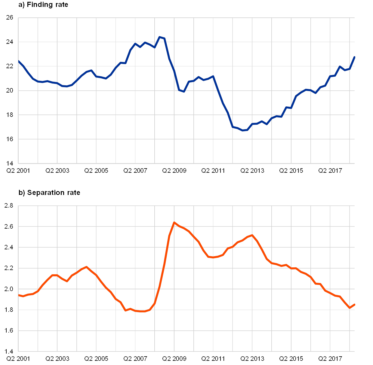
The main cause of the outward shift of the euro area Beveridge curve appears to be a decrease in the job finding rate. During the crisis the job separation rate increased and the job finding rate decreased. However, when the Beveridge curve shifted in 2011, the decrease in the job finding rate was more pronounced than the increase in the separation rate (see Chart 2), thus largely contributing to the outward shift of the Beveridge curve.[19] The weakness in the finding rate can be explained by lower matching efficiency (see Section 3). Overall, the analysis of job flows shows that inward or outward shifts of the Beveridge curve can have a business cycle component, as described in Elsby et al.[20]
Chart 1
The Beveridge curve for the euro area and for the five largest euro area countries
(x-axis: unemployment rate; y-axis: job vacancy rate)

Sources: Eurostat and ECB staff calculations.
Notes: For the euro area the job vacancy rate series is standardised by its mean and standard deviation. For each of the countries the job vacancy rates are adjusted for statistical breaks. All six series are four-quarter moving averages.
Chart 2
Labour market flows
(finding rate: as a percentage of the unemployed; separation rate: as a percentage of the employed)
Sources: Eurostat and ECB staff calculations.
Notes: Labour market flows are computed based on Shimer in that movements to and from unemployment are estimated based on information on unemployment duration – see Shimer, R., “The Cyclical Behaviour of Equilibrium Unemployment and Vacancies”, American Economic Review, Vol. 95, No 1, 2005, pp. 25-49. Flows to and from inactivity are assumed constant. The latest observations are for the third quarter of 2018. Eurostat has published data on flows since the second quarter of 2010 (data are available for the five the largest euro area countries except Germany). The analysis of these data shows that there have not been significant changes in the flows from unemployment to inactivity, while flows from inactivity to unemployment increased in Italy and France, but decreased in Spain.
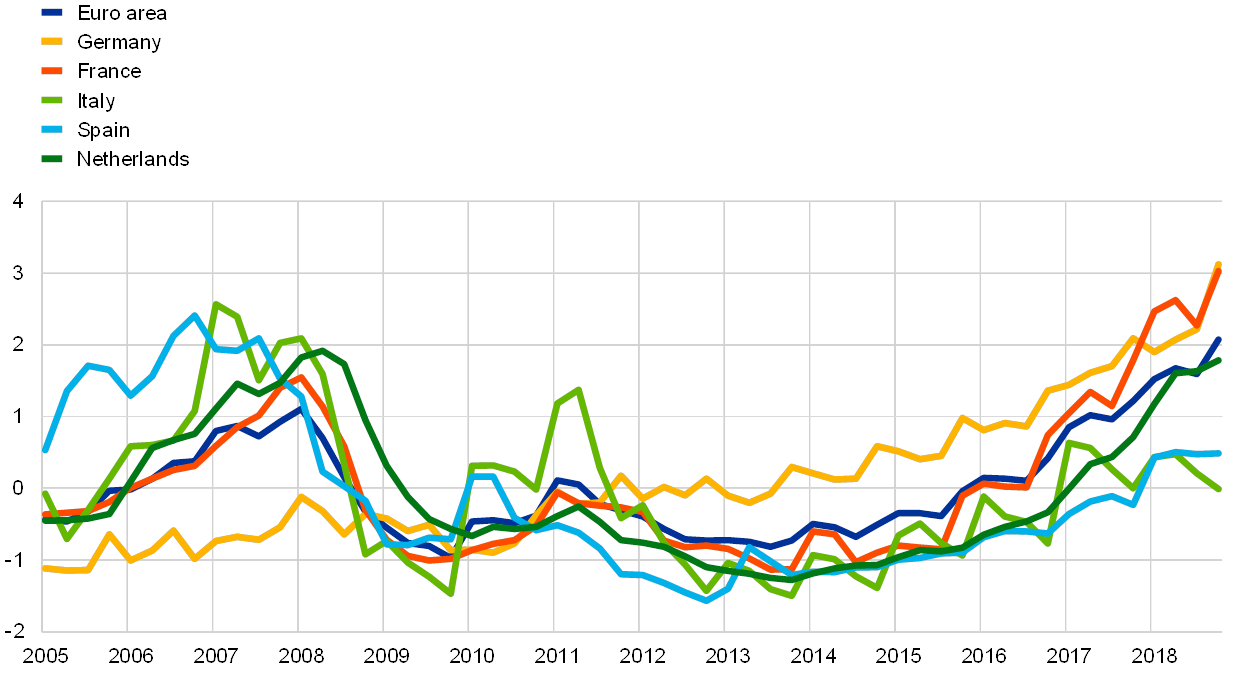
Job vacancy rates are at a very high level, while the finding rate is yet to reach previous peaks and unemployment remains above previous lows. This suggests both increased tightness and lower efficiency in the labour market. Labour market tightness at the aggregate euro area level is substantially higher than before the crisis, but there is large heterogeneity across countries (Chart 3). In Germany, the vacancy-unemployment ratio has quadrupled since 2006 and is the major determinant of the labour market tightness observed at the aggregate euro area level. In addition, in France labour market tightness is higher than before the crisis and has increased rapidly in the last two years. On the contrary, in Spain and Italy labour market tightness is significantly below previous peaks. At the aggregate euro area level, labour market tightness has been above pre-crisis levels since the third quarter of 2017. Meanwhile, labour market tightness in the United States reached pre-crisis highs in the second quarter of 2015.
Chart 3
Labour market tightness
(standardised values of the ratio of vacant posts to unemployed persons)
Sources: Eurostat and ECB staff calculations.
Note: The latest observation is for the fourth quarter of 2018.
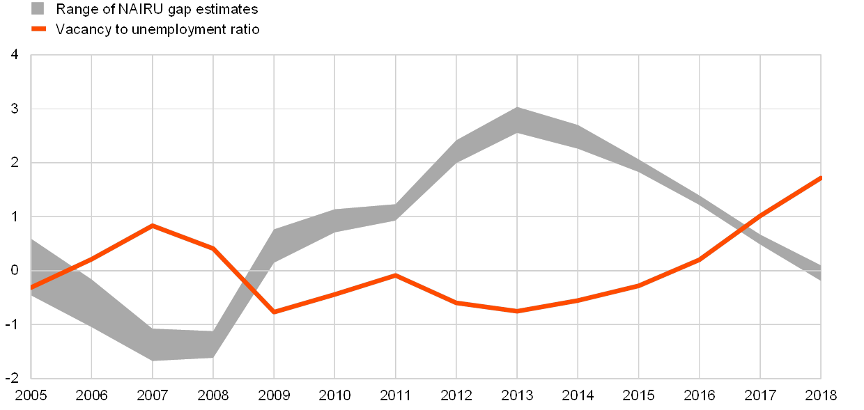
The vacancy-unemployment ratio provides similar information to standard measures of labour market slack. The vacancy-unemployment ratio tends to capture cyclical conditions in the labour market from a quantitative perspective by balancing out the effects of labour demand and supply. This measure is similar to other commonly used measures of the unemployment gap derived using the Phillips curve framework (see Chart 4 for a comparison). In the wage Phillips curve, the derived non-accelerating wage rate of unemployment (NAWRU) is assumed to implicitly embed labour market mismatch. The information content extracted from the analysis of the Beveridge curve, on the other hand, can disentangle labour market tightness from efficiency. In doing so, job matching efficiency complements labour market tightness with a qualitative margin (see Section 3) and thus may provide richer information on the dynamics of wages.
Chart 4
Labour market tightness and the non-accelerating inflation rate of unemployment (NAIRU) gaps
(annual averages; range of NAIRU gap estimates are in percentage points; tightness is measured as the z-score)
Sources: Eurostat and ECB staff calculations.
Notes: Tightness refers to the aggregation of the five largest countries in the euro area. The NAIRU gap estimates used are those computed by the European Commission, the IMF and the OECD and are defined as the difference between the actual unemployment rate and the respective NAIRU estimates.
Box 1 The Beveridge curve for the US labour market
This box looks at unemployment rate developments in the United States from the perspective of the relationship between the unemployment rate and the vacancy rate, which is represented by the Beveridge curve. The unemployment-vacancy relationship appears to be an informative tool, given that it can give a broad indication of whether changes in the unemployment rate are caused solely by cyclical developments in economic activity or by more permanent or structural factors.
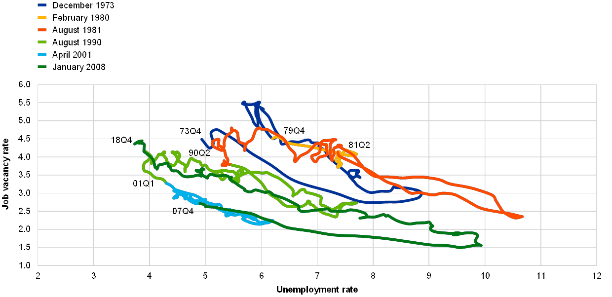
Developments in the US Beveridge curve since the 1970s point to efficiency gains as the dominant factor in the unemployment-vacancy relationship. Past developments in the US Beveridge curve illustrate the presence of both activity shocks and structural shocks (see Chart A). Anticlockwise loops reflecting activity shocks can be clearly identified starting (following the recessions) in 1973, 1981, 1990 and 2008, with much shorter ones in 1980 and 2001. In all cases, the vacancy rate followed a downward pattern in the recessionary part of the cycle, while the unemployment rate grew, with the reverse occurring in the expansionary phase. However, it is worth noting that, together with activity shocks, shifts in the unemployment-vacancy relationship have taken place since the 1970s. In particular, an initial outward shift between 1973 and 1980 was more than compensated for by an inward shift between the 1980s and the 2000s, which points to the dominant role of positive structural shocks in the US labour market, i.e. shocks leading to an increase in the effectiveness of the job matching process.
Chart A
The US Beveridge curve
(as a percentage of the civilian labour force; three-month moving averages)
Source: FRED database.
Notes: Different colours refer to different cycles, starting from NBER-dated recessions. JOLTS vacancy data are extended using the composite Help-Wanted Index constructed in Barnichon R., “Building a composite Help-Wanted Index”, Economics Letters, Vol. 109, No 3, 2010, pp. 175 -178. The latest observation is for December 2018.
Developments since the global financial crisis point primarily to cyclical shocks. A very deep recession brought the unemployment rate to levels not seen since the early 1980s and the vacancy rate to historical lows. This was followed by a particularly long and slow expansion in historical terms. From the labour market perspective this implied less-smooth changes in both the unemployment rate and the vacancy rate compared with previous cycles, although the unemployment rate still reached record lows at the end of 2018 and the vacancy rate was close to historical highs. There has been some discussion as to whether the Beveridge curve has shifted slightly in the current business cycle, particularly at the early stages of the recovery, but there is a broad consensus that some friction in the matching process after recessions is visible in most recovery phases without implying a sustained rise in structural unemployment.[21] Indeed, most estimates point to a decline in structural unemployment in the United States over the last few years.[22]
3 Measuring labour market efficiency
In this section we derive measures of labour market efficiency for the euro area to further the analysis of the labour market and wage dynamics. As discussed in the previous sections, the Beveridge curve framework requires labour market tightness to be complemented with a measure of efficiency to provide a more comprehensive picture of the euro area labour market. In this section the assessment of the cyclical position of the labour market will therefore require information derived from labour market tightness and labour market efficiency. These two measures are important for assessing the overall strength of the labour market and for understanding how they jointly affect wage developments.
Two empirical measures of labour market efficiency can be derived from the Beveridge curve and the job finding rate. In the simple theoretical framework presented in Box 2, the matching efficiency affecting the job finding rate is the only underlying factor generating a shift of the Beveridge curve. In practice, the Beveridge curve may also shift for reasons other than matching efficiency. Therefore, measures of efficiency based on the Beveridge curve and measures of efficiency based on the finding rate (matching function) may ultimately differ. Comparing these two approaches helps to increase the robustness of the exercise. This empirical exercise comes with a number of caveats as data on vacancies and job flows have a relatively short time span and, in the context of the euro area, there are no micro data available for a more granular analysis of the labour market (as in Şahin et al.[23]). Nevertheless, this is a useful exercise as it may provide a more comprehensive view of labour market adjustment in the euro area and highlight new implications for euro area wage dynamics.
A first measure of matching efficiency can be derived by recalling the aggregate matching function and using the job finding rate. Following the work of Petrongolo and Pissarides[24], the matching function is specified as a constant returns to scale Cobb-Douglas function of the vacancy rate and the unemployment rate. The aggregate matching function can be estimated by looking at the quarterly job finding probabilities ( ) and the vacancy-unemployment ratio (market tightness).[25] The outflows from unemployment ( ) are measured following Shimer[26], while market tightness is derived using the break-adjusted vacancy rate.[27] The matching efficiency is therefore defined as the residual from estimating a reduced-form matching function[28]
where the vacancy-unemployment ratio is usually defined as labour market tightness, .
An alternative measure of job matching efficiency can be derived by estimating the elasticity between vacancies and unemployment. Such a measure directly reflects the shifts in the Beveridge curve while also accounting for the negative relationship implied by the vacancy to unemployment ratio (i.e. market tightness), specified as follows:
Empirically, such a crude measure of labour market efficiency features both an outward shift and a steepening of the slope. As shown in Chart 1, the euro area Beveridge curve has also become steeper following the post-2011 outward shift.[29] The derived residual after estimating a constrained regression[30] between the vacancy rate and the unemployment rate provides a time series for labour market efficiency which can proxy the side-shifts of the Beveridge curve between the second quarter of 2004 and the first quarter of 2018.
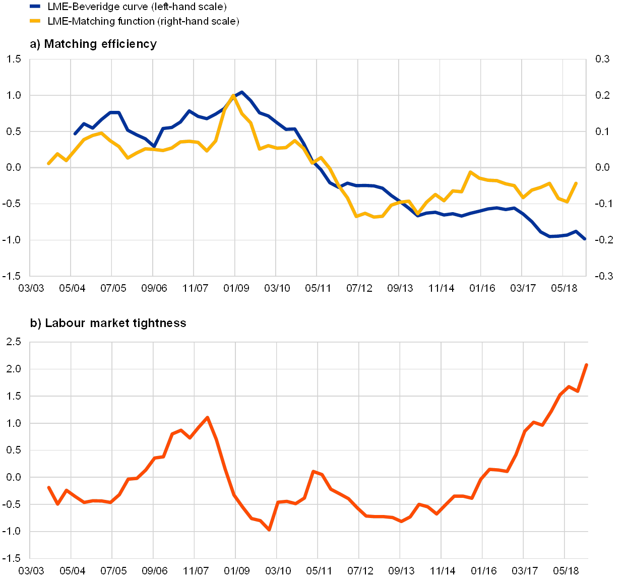
According to these measures, matching efficiency deteriorated during the crisis (see Chart 5). These two efficiency measures are closely related but they do display some differences. The matching efficiency derived from the Beveridge curve (equation 2) tends to be more comprehensive than that derived using the matching function (equation 1). While the method based on the matching function directly captures the matching process, the Beveridge curve efficiency measure also captures the dynamics of job separations as well as potential labour force movements from inactivity to the labour market. Overall, the correlation between these two measures is relatively high and the information content is consistent. These two measures indicate that labour market efficiency has not fully recovered compared with pre-crisis times. According to the search and matching model sketched in Box 2, the information on the functioning of the labour market (efficiency) complements the purely quantitative indicator of labour market tightness. In the pre‑2008 period matching efficiency and tightness were positively correlated (see Chart 5), a situation which, all other things being equal, can lead to higher wages. By contrast, more recently efficiency and tightness have been moving in opposite directions, leading to counterbalancing effects on wages.
Chart 5
Measures of matching efficiency
(a) measures of labour market efficiency (LME) are in percentage points; b) labour market tightness is the z-score of the vacancy -unemployment ratio)
Sources: Eurostat and ECB staff calculations.
Notes: Measures of labour market efficiency are based on equations (1) and (2) respectively. Labour market tightness is the ratio of the GDP-weighted aggregate vacancies for the five largest euro area countries to the respective seasonally adjusted unemployment rate. Vacancies are break-adjusted and standardised by their country-specific mean and standard deviation.
The heterogeneity of the unemployment pool and the dispersion of unemployment across countries may have had a negative impact on matching efficiency. During the crisis the unemployment pool became more heterogeneous. The unemployment rate of low-skilled workers also grew significantly and still remains far above the unemployment rate of medium and high-skilled workers (see panel (a) of Chart 6). This type of imbalance between skill supply and skill demand causes the unemployment rate and the job vacancy rate to rise simultaneously, shifting the Beveridge curve to the right. At the same time, the dispersion of the unemployment rate increased across countries (see panel (b) of Chart 6). The geographical dispersion in unemployment and vacancies has led to a situation in which there is a high number of vacancies in some local labour markets at the same time as high unemployment in other labour market segments, which reduces the response of unemployment to vacancies. Barnichon and Figura[31] show that matching efficiency declines when the average characteristics of the unemployed deteriorate substantially, or when dispersion in labour market conditions increases markedly. These two factors occurred in the euro area during the crisis: not only did low-skilled unemployment rates increase substantially, the dispersion of the unemployment rate also increased.[32]
Chart 6
Composition and dispersion of the unemployment rate
(a) percentages; b) coefficient of variation)

Sources: Eurostat and ECB staff calculations.
Notes: The unemployment rate by skill level is based on the aggregation of unemployment rates across the five largest euro area countries. The coefficient of variation is computed for the five largest euro area countries.
Box 2 Labour market efficiency in a search and matching model
This box provides an overview of the Beveridge curve and how it is derived from a simple search and matching model. This framework allows for the joint determination of an unemployment rate, a vacancy rate and a real wage that are mutually consistent. In fact, an analysis of the Beveridge space (the vacancy-unemployment diagram) in itself does not provide enough information to pin down the dynamics of wages, productivity and labour demand and has to be enriched with (i) a firm job creation condition and (ii) a wage setting mechanism. We therefore follow a simpler version of the model developed by Mortensen and Pissarides[33] to provide a coherent narrative of the fluctuations in unemployment, vacancies and wages.[34]
This framework offers a simple yet coherent tool to analyse possible movements in the Beveridge space. Changes in the Beveridge space can reflect movements in market tightness and shifts in job matching efficiency. Market tightness movements are characterised by a negative relationship between vacancies and unemployment, and shifts in job market efficiency by a positive relationship. Both market tightness and matching efficiency can play an important role in the determination of wages. The framework introduced in this box can account for the driving forces behind changes in the Beveridge curve and can also be helpful in rationalising the effects on wages.[35]
Equilibrium conditions from a search and matching model
A simple description of the search and matching model with constant (exogenous) job destruction rates – following Pissarides[36] – can be summarised by three equilibrium conditions for the main variables of interest: unemployment rate, , vacancy rate, , and real wages, :
with exogenous destruction rates, , search costs, , bargaining power of the worker, , unemployment benefits, , productivity, , and the discount rate, . The variable is usually defined as market tightness as it reflects the relative strength between labour demand and labour supply factors, which are proxied by the number of vacancies and the number of people searching for a job, respectively. The function is a transformation of the matching function.[37]
The first equation ( ) is the Beveridge curve, which describes the relationship between the vacancy rate and the unemployment rate and is derived from a steady-state condition on job flows in and out of the unemployment pool.[38] The second equation ( ) refers to the job creation condition based on the assumption that firms will keep posting vacancies as long as the marginal job has a non-negative present discount value. The third equation ( ) refers to the Nash solution to the wage bargaining problem of sharing the surplus generated by the job match between a worker and a firm. Both and depend on the matching function , which is not the case for the equation.[39]
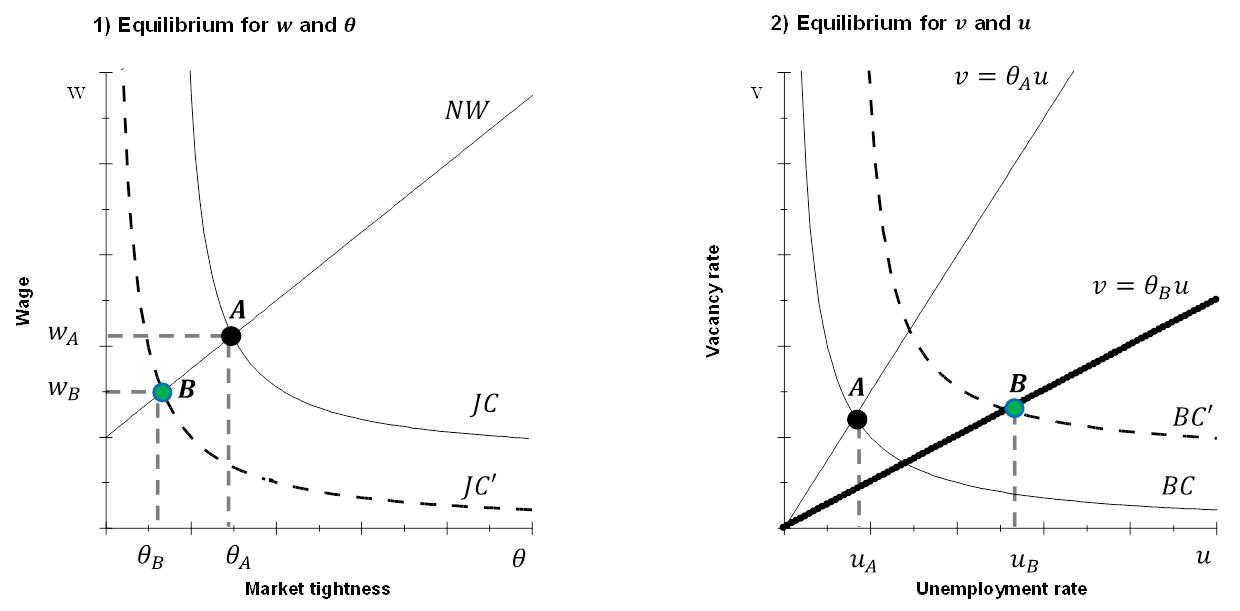
Figure A.1 and A.2 display these three equations to provide a visual representation of the behaviour of and . These three equations jointly provide a simple yet consistent framework for analysing the dynamics of the Beveridge curve and wages. As these equations show, all three theoretical relationships are needed and it is not possible to consider the implications for wages using the Beveridge space alone. Figure A.1 shows the space and the equilibrium arising from the intersection between the job creation condition, , and the Nash wage equation, , point A. Figure A.2 shows the space and the equilibrium arising from the intersection between the Beveridge curve and market tightness line where is derived from Figure A.1.
The model can account for the following possible exogenous drivers of labour market fluctuations: (i) productivity, (ii) job matching efficiency, (iii) worker’s outside option and bargaining power, and (iv) job-posting search costs.
Job matching efficiency
In view of the empirical analysis undertaken in Section 3 of this article, the focus will be on providing a theoretical description of a job matching efficiency shock under the search and matching framework. Such a diagrammatical description can also be viewed as a simple description of an impulse response function in a theoretical macro model of equilibrium unemployment.
In this framework, a job matching efficiency shock affects the curve and the curve via the matching function. Figure A.1 shows the space that includes the job creation condition and the Nash wage equation . The intersection point A is the equilibrium . An exogenous shift in efficiency generates a downward translation of the job creation conditions curve . For instance, if efficiency were to decrease, both and would decrease and the ratio would increase. All other things equal, wages and would decrease.[40] An extension of the model with endogenous job destruction rates – in which depends on the level of productivity of the job match – would suggest an even larger increase in this ratio as lower productivity matches will feature higher destruction rates. This would further compress the wage offered in the job creation condition. This discussion highlights that there may be an important labour demand channel when accounting for the effects of job matching efficiency. In a more general set-up, a higher skills mismatch in the labour market could affect the productivity of a job match and drive down the wages firms are willing to offer.
Figure A
A basic search and matching model
Source: Author’s elaboration.
Note: Based on Pissarides, C.A., op. cit.
Turning to Figure A.2, the upward linear curve follows the definition of tightness and has the slope which is determined in Figure A.1. The downward-sloping curve is the equation. A shift in job matching efficiency will affect both curves. The Beveridge curve will shift outward because of the lower job finding probability. The linear curve will flatten following the reduction in the tightness from shown in Figure A.1. This implies that the change in the unemployment rate is amplified by the change in .
To conclude, a negative efficiency shock will lead to lower market tightness, , lower wages and higher unemployment. The effect on the vacancy rate remains undefined and depends on the final parameterisation of the full model.
Box 3 Labour market tightness and efficiency in the wage Phillips curve
This box aims to clarify whether the combination of labour market tightness and matching efficiency can help to explain wage growth in the euro area in an augmented Phillips curve. It is still unclear as to why wages grew only moderately from 2013 to 2017 despite a notable reduction in the unemployment rate of the euro area. The original Phillips curve suggested a simple inverse relationship between wage growth and the unemployment rate, i.e. the lower the unemployment rate, the higher the rate of wage growth.[41] More recent specifications of the wage Phillips curve, as, for example, in Galí[42], are more complex; they suggest that nominal wage growth is determined by the cyclical stance of the economy, inflation expectations and productivity growth developments. The equilibrium conditions of a simple version of the search and matching model suggest that an additional factor is necessary to fully describe the changes in the vacancy-unemployment space. Job market efficiency measures should therefore be included in the wage Phillips curve given that, empirically, labour market tightness and efficiency may produce different information over the business cycle.
The precise functional form of the wage Phillips curve (for example in terms of lag structure or linearity vs non-linearity) and the chosen determinants remain subject to discussion. One way to hedge against such model uncertainty is to use a large set of proxies for the labour market cycle, inflation expectations and productivity growth.[43] This box shows the results for a set of wage Phillips curves that alternate 18 slack measures (including unemployment rate, unemployment gap from various institutions (ECB, IMF, OECD), and job market tightness), 16 inflation expectations measures (including those collected by Consensus Economics and in the ECB Survey of Professional Forecasters (SPF), and lagged headline inflation) and the measures of job market efficiency.[44] One-third of the specifications are standard, without a job market efficiency measure, one-third include the job market efficiency measure derived from the Beveridge curve and one-third include the measure derived from the matching function.
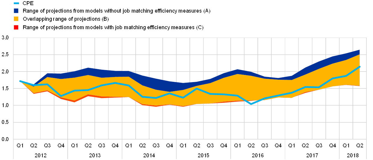
Measures of matching efficiency help to explain past moderate wage developments in the euro area. According to a measure of fit (Schwarz info criterion) some of the best specifications include the job market efficiency measures. Chart A shows the range of the paths of compensation per employee obtained using the wage Phillips curve models and conditioning on the path of slack, productivity, and past or expected inflation starting in 2012. When job market efficiency measures are added to the wage Phillips curves there is a marginal downward shift of the range of projections compared to the baseline models that do not include these measures. This suggests that the job market efficiency measures may be useful in explaining the moderate wage growth in the euro area over the last eight years, albeit to a rather limited extent.
Chart A
Euro area: conditional forecast of annual growth of compensation per employee (CPE)
(year-on-year changes)
Source: ECB calculations based on data from Eurostat, the IMF, Consensus Economics and the SPF.
Notes: Results are based on a thick modelling approach that includes a broad range of fixed coefficient specifications of the Phillips curve including or excluding job market inefficiency measures. The parameters are estimated over the sample period 2005Q1-2018Q2. The conditional out-of-sample forecast is carried out for the period 2012Q1-2018Q2. The ranges depict forecasts for the growth of compensation per employee coming from differently specified Phillips curves. The specifications include permutations across the expectation formation (backward or forward-looking), the variables representing slack and the job matching efficiency (JME) measures. In the chart the range of projections of the models without JME measures is represented by the blue and yellow area (A+B) while the range of projections from models that include JME measures is represented by the yellow and red area (B+C).
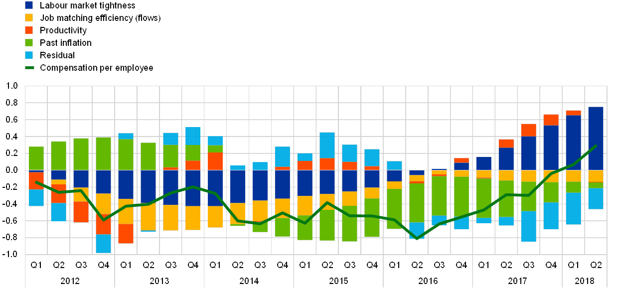
The decomposition of the contribution of the exogenous variables confirms that a decline in job market efficiency has a dampening effect on wages. Chart B shows the contribution of the exogenous variables to wage growth (as a deviation from the long-run mean) for a specification that includes job market tightness and matching efficiency. From 2012 to 2015 cyclical developments measured by job market tightness explain most of the lower-than-average developments in wages, while in 2017 and 2018 the contribution becomes positive. Job market inefficiency has a dampening effect on wages over the full period, and in particular in 2013 and 2014. A very important additional driver of low wage growth is low inflation, particularly in 2016. Similar results can be obtained using only the unemployment rate, with the contribution of this variable corresponding to the combined impact of job market tightness and matching efficiency.
Chart B
Euro area: contribution of different exogenous variables according to a wage Phillips curve
(percentage points)
Source: ECB staff calculations.
Notes: The green line shows deviations of year-on-year growth of compensation per employee from its long-run mean. Contributions (including residuals) are also shown as deviations from their long-run mean. Contributions are calculated based on an equation in which compensation per employee (the annualised quarterly growth rate) is regressed against its own lag, a measure of slack (job market tightness), the job matching efficiency measure derived from the residuals of the job market matching function, productivity growth, the four-quarter moving average of headline inflation and a constant. Past developments of these variables impact current compensation per employee through lagged compensation per employee. In the chart these contributions are associated with the single exogenous variables despite showing a generic contribution of lagged compensation per employee.
The results suggest that, despite some caveats, job market efficiency measures help to explain past moderate wage growth in the euro area. The caveats relate to the fact that the analysis does not allow for a structural interpretation of shocks that would explain wage developments, i.e. there is not necessarily a causal relationship between the explanatory variables depicted in Chart B and low wages, as they could simply be reacting to the same common shocks. Also, the reliability of these results is affected by the low number of observations available for these measures and, therefore, the length of the estimation sample. Although this framework provides a useful and complementary perspective for understanding wage developments, and may help to partially explain past moderate wage developments in the euro area, the overall quantitative implications for wages are largely consistent with those of the standard Phillips curve approach.
4 Concluding remarks
The article analyses the main patterns of the Beveridge curve and highlights the importance of both labour market tightness and labour market efficiency. The Beveridge curve seems to have significantly shifted outwards in the euro area, with the unemployment rate approximately similar to the pre-crisis period and the job vacancy rate currently significantly higher. Our empirical findings show that there has been a significant deterioration in aggregate matching efficiency since the start of the crisis. The deterioration in matching efficiency is not necessarily structural and contains useful cyclical information that can be used to assess the state of the labour market and possible implications for wage developments. We show that lower matching efficiency may have marginally contributed to weaker wage dynamics. This framework therefore helps to enhance our understanding of unemployment and wage fluctuations. However, the quantitative implications for wages presented in this article differ only marginally from those of the standard Phillips curve approach.
The reasons behind the sharp decline in matching efficiency require further investigation into the heterogeneity and composition of the labour market. According to recent studies, the two main factors driving the decline in matching efficiency are the increased heterogeneity of the unemployment pool and the increased dispersion of unemployment rates across countries. However, other factors may be at play. First, the dynamics of the labour force and its composition may also affect labour market efficiency. The euro area labour force participation rate has increased steadily since the early 2000s but has grown at a lower than average rate since the crisis. Therefore, in the context of the euro area Beveridge curve analysis, the outward shift in 2011 cannot be linked to the movements of the participation rate. Second, the role of sectoral reallocations may also have contributed marginally to the outward shift of the Beveridge curve as reallocations are usually associated with a significant spike in job separation rates. However, the timing of the outward shift of the Beveridge curve cannot really be linked to the slight change in the euro area job separation rate in 2011.
- A simple description of this framework is presented in Chapter 1 of Pissarides, C. A., Equilibrium unemployment theory, 2nd edn., The MIT Press, Cambridge, Massachusetts, 2000.
- In this article two concepts of efficiency will be used, almost interchangeably. Matching efficiency is strictly related to the efficiency of the matching process (derived from the matching function – see Section 3 and Box 2). Labour market efficiency is a broader concept that includes matching efficiency and relates to side-to-side shifts of the Beveridge curve.
- Blanchard, O.J. and Diamond, P., “The Beveridge Curve”, Brookings Papers on Economic Activity, Vol. 1989, No 1, 1989, Washington DC, pp. 1-76.
- Bova, E., Jalles, J.T. and Kolerus, C., “Shifting the Beveridge curve: What affects labour market matching?”, International Labour Review, Vol. 157, No 2, 2018, pp. 267-306.
- Elsby, M.W.L., Michaels, R. and Ratner, D., “The Beveridge curve: a survey”, Journal of Economic Literature, Vol. 53, No 3, 2015, pp. 571-630.
- Barnichon, R. and Figura, A., “Labor Market Heterogeneity and the Aggregate Matching Function”, American Economic Journal: Macroeconomics, Vol. 7, No 4, 2015, pp. 222-249.
- Şahin, A., Song, J., Topa, G. and Violante, G.L., “Mismatch Unemployment”, American Economic Review, Vol. 104, No 11, 2004, pp. 3529–3564.
- See the work by Petrongolo, B. and Pissarides, C.A., “Looking into the Black Box: A Survey of the Matching Function”, Journal of Economic Literature, Vol. 39, No 2, 2001, pp. 390-431.
- The counterbalancing flow to the job finding rate is the job separation rate, which measures the outflows from employment to unemployment.
- Here, the concept of job matching efficiency is similar to the concept of efficiency of the production function, as measured by total factor productivity.
- See Crump, R.K., Eusepi, S., Giannoni, M. and Şahin, A., “A Unified approach to measuring u*”, Brookings Papers on Economic Activity, BPEA conference drafts, 2019.
- The short length of the job vacancy rate series in the euro area means that a longer-term Beveridge curve, such as that for the US labour market in Box 1, cannot be produced.
- Eurostat provides information and the dates on which national statistics offices changed their statistical methodology for measuring vacancies.
- The job vacancy rates adjusted for statistical breaks were standardised by their respective historical average and standard deviation. The aggregation of the country series is weighted by the share of GDP. As a robustness check, the share of the labour force has also been considered, but it had no impact on the overall results of the EA-5 Beveridge curve.
- For presentational reasons we mainly focus on the five largest euro area countries. This is sufficient to illustrate some relevant heterogeneity in the aggregate euro area data.
- Similar data on labour shortages have been used for Beveridge curve analyses in other works, namely in Anderton, R. et al., “Comparisons and contrasts of the impact of the crisis on euro area labour markets”, Occasional Paper Series, No 159, ECB, Frankfurt am Main, February 2015; and Bonthuis, B., Jarvis, V. and Vanhala, J., “What’s going on behind the euro area Beveridge Curve?”, Working Paper Series, No 1586, ECB, Frankfurt am Main, September 2013.
- The U6 is a broader measure of unemployment that includes all individuals falling under one of the following categories: unemployed, available but not seeking work, seeking work but not available, and working part-time but would prefer more hours (underemployed workers).
- Diamond, P. and Şahin, A., “Shifts in the Beveridge curve”, Research in Economics, Vol. 69, No 1, 2015, pp. 18-25.
- Elsby, Hobijn and Şahin find that variation in the job finding rate explains 85% of the overall variation in the unemployment rate for Anglophone countries, while for continental European countries they estimate that only 55% of the overall variation in the unemployment rate is accounted for by the variation in the job finding probabilities – see Elsby, M.W.L., Hobijn, B. and Şahin, A., “Unemployment Dynamics in the OECD”, Review of Economics and Statistics, Vol. 95, No 2, 2013, pp. 530–48. Robert Shimer instead finds that job finding probability accounted for three-quarters of the fluctuations in the unemployment rate in the United States during the period 1948-2010 – see Shimer, R., “Reassessing the ins and outs of unemployment”, Review of Economic Dynamics, Vol 15, No 2, 2012, pp. 127-148.
- Elsby, M.W.L., Michaels, R. and Ratner, D., op. cit.
- For a discussion on the interpretation of outward shifts of the Beveridge curve, see Diamond, P. and Şahin, A., op. cit.
- From 5.1% in 2011 to 4.6% in 2018 according to Congressional Budget Office estimates.
- Şahin, A., Song, J., Topa, G. and Violante, G.L., op. cit.
- Petrongolo, B. and Pissarides, C.A., op. cit.
- See also Arpaia, A., Kiss, A. and Turrini, A., “Is unemployment structural or cyclical? Main features of job matching in the EU after the crisis”, European Economy – Economic Papers, No 527, European Commission, September 2014.
- See Shimer, R., The Cyclical Behaviour of Equilibrium Unemployment and Vacancies, op. cit.
- In the same way as for the vacancy rate, job vacancies have also been adjusted following the description of structural breaks related to statistical changes in the measurement of job vacancies provided by Eurostat.
- The estimation has been performed using the ordinary least squares (OLS) and generalised method of moments (GMM) methods on the logs of the Cobb-Douglas matching function. For the GMM method, lags of the vacancy and unemployment rate have been used as instruments.
- Such an equation is also estimated by imposing a coefficient restriction which finds the average of the slope of the Beveridge curve before and after 2011.
- For robustness, the average elasticity between vacancies and unemployment before and after 2011 is used. The derived matching efficiency measure is on the whole robust to statistically small changes.
- Barnichon, R. and Figura, A., op. cit.
- Beyer and Smets show that labour mobility is a less important adjustment channel in response to shocks, with the unemployment rate playing a more persistent role – see Beyer, R.C.M. and Smets, F., “Labour market adjustments in Europe and the US: How different?”, Economic Policy, Vol. 30, No 84, 2015, pp. 643-682.
- Mortensen, D.T. and. Pissarides, C.A., “Job Creation and Job Destruction in the Theory of Unemployment”, The Review of Economic Studies, Vol. 61, No 3, 1994, pp. 397-415.
- For a theoretical overview, see Pissarides, C.A., Equilibrium Unemployment Theory, op. cit.
- See Elsby, M.W.L., Michaels, R. and Ratner, D., op. cit.; and Shimer, R., “Mismatch”, American Economic Review, Vol. 97, No 4, 2007, pp. 1074-1101.
- Pissarides, C. A., op. cit.
- The matching function is defined as where is matching efficiency and , and .
- The current model specification does not account for flows in and out the inactivity pool of the working age population.
- This means that the curve does not shift following a job matching efficiency shock.
- This ratio can be interpreted as the average expected search cost of posting a vacancy. If firms keep posting vacancies and the market (the matching function) does not make enough job matches, firms will have to bear higher search costs or increase the search effort to fill their vacancies. In net present value terms, these higher costs from search and matching will negatively affect the strength of labour demand and the wage offered.
- Phillips, A.W., “The Relation between Unemployment and the Rate of Change of Money Wage Rates in the United Kingdom, 1861-1957”, Economica, New Series, Vol. 25, No 100, 1958, pp. 283-299.
- Galí, J., “The Return of the Wage Phillips Curve”, NBER Working Papers, No 15758, 2010. The standard New Keynesian model with staggered wage setting implies a simple dynamic relation between wage inflation and unemployment. Galí finds that, even under the strong assumption of a constant natural rate of unemployment, this simple relation accounts reasonably well for the co -movement of wage inflation and the unemployment rate in the United States.
- This thick modelling approach is similar to the one applied for the price Phillips curve in Ciccarelli, M. and Osbat, C., “Low inflation in the euro area: Causes and consequences”, Occasional Paper Series, No 181, ECB, Frankfurt am Main, January 2017, and in the article entitled “Drivers of underlying inflation in the euro area over time: a Phillips curve perspective” in this issue of the Economic Bulletin.
- Wage Phillips curves are specified as a regression of nominal compensation per employee (expressed in terms of annualised quarter-on-quarter growth) on its own lag, the first lag of a measure of labour market slack, productivity growth, a measure of expected inflation, the intercept, and the measures of job market efficiency. We estimate a total of 864 specifications.


